
As a spreadsheet application, Microsoft® Excel is used to enter text and numbers to be organized, calculated, and analyzed. Entering formulas allow any changes in the original numbers to be automatically recalculated throughout an entire worksheet. Data may be formatted creating an attractive, readable presentation of tables or charting, and text manipulation features produce attractive and informative reports.
By following the steps outlined in this overview, a basic understanding of Microsoft® Excel should be achieved. Although examples in this overview reference Microsoft® Excel 2007, fundamental concepts should be relatively easy to apply to other versions of Excel.
The Worksheet and Cells
Microsoft® Excel is a spreadsheet application. Work performed in Excel is done on a worksheet which is a grid of rows and columns. The rows are numbered along the left of the grid while the columns are headed by letters along the top. Each intersection of a row and a column is called a cell and has a unique reference identifying it. For example, the cell where column B and row 5 intersect is cell B5. Cells are used to store data such as labels and numbers, and cell references are used when writing formulas or referring to cells.
Data is entered into single cells. The cell that has been selected to enter data is called the active cell and is identified by a heavy border.

Changing the Active Cell
To change the active cell, move the mouse pointer into a cell and click. For example, if we wanted B4 to be the active cell, simply click that cell. Upon selecting B4, the formula bar would display the contents of that cell or, in the illustration above, 67800. Demonstrated in the illustration is cell E4 as the active cell and the formula =C4/D4 displayed in the formula bar since the contents of cell E4 is the formula dividing the contents of C4 or $489,000.00 by D4 or $225,000.00.
Scrolling Through the Worksheet
There are several methods that can be used to scroll through the worksheet:
- Move the pointer to the down arrow in the vertical scroll bar on the right edge of the window and click. The worksheet scrolls down.
- Move the pointer to the right arrow in the horizontal scroll bar on the bottom of the window and click. The worksheet scrolls to the right.
- Click, hold and drag either the vertical or horizontal scroll bars. This scrolls through the worksheet for as long as you hold the scroll bar.
Entering and Editing Data
Entering Data
As previously pointed out, data is entered by selecting a cell and entering the data. In the illustration below, if you wanted to enter the year column (column A) you would click on cell A2, type 2011 and press [ENTER]. Entering the data would automatically advance the active cell to the next row or cell A3.
The reason A2 in the illustration below was chosen as the first cell to start entering the year labels is to allow a row (row 1) to be used for headings of each of the columns. Subsequently, columns B, C, D, etc., were entered. This was done by first entering the column heading, e.g., Net Income, and then the values 80000, 78900, 67800, etc. Note the values entered were “plain” numbers such as 80000 instead of the formatted number $80,000.00. It is important to enter the number as a plain number and format the cell to the required specification. We will do this later.

Editing Data
Once you have entered data into a cell, that data can be edited by first clicking on the cell to make the cell active and then clicking on the formula bar above the worksheet. This allows you to insert or delete characters in that cell. An alternate method of editing the contents of a cell is to click on the cell to make it the active cell and then press the [F2] function key at the top of the keyboard. You can delete the contents of a cell by clicking on the cell and pressing [Delete] on the keyboard.
Inserting Columns, Rows, and Cells
To insert a column, click anywhere in a column you wish the new column to appear ahead of or to the left of, and then on the Home tab, in the Cells group, on the Ribbon at the top of the Excel screen, click the arrow by Insert, and then click Insert Sheet Columns. Selecting an existing row to insert a new row ahead of or above is done the same way.

When you click the arrow on the Insert button, you will notice the options to Insert Cells, Insert Sheet Rows, Insert Sheet Columns, or Insert Sheet. When requesting a new cell, Excel asks if you wish to move the existing cells to the right or down.
Working with Formulas
The power of a spreadsheet application is demonstrated most clearly by formulas. Formulas can be simple, like dividing the values in two cells, or they can be very complex. The scope of this overview will focus on a more simple example of working with formulas.

Entering and Editing Formulas
A formula can always be identified because it starts with an equal sign (=). To enter a formula, click on the cell that is to contain the formula and start the formula by pressing the equal sign (=). This tells Excel to handle the contents as a formula instead of a label or simple text. In cell E2 (1.724137931) in the illustration above, we entered the formula =C2/D2. After pressing [ENTER], Excel automatically advanced to cell E3. Cell E2 displayed the results of the formula or 1.724137931. The formula =C2/D2 is still the content of the cell, only Excel has displayed the result of the formula.
In our illustration above, to determine Total Assets Turnover for each year, we would continue entering formulas into each cell in column E referencing the cells for Sales divided by Total Assets for each year.
As stated, when a cell contains a formula, the value produced by that formula is displayed, as in cell E2 in the illustration above. The formula itself, however, is displayed in the formula bar above the worksheet. Once the formula is entered in the cell, it will be displayed only if the cell is being edited. Again, to edit a cell, click on the cell making it the active cell and either click on the formula bar above the worksheet, or press the [F2] function key at the top of the keyboard.
Copying Formulas Between Cells
Since our example is relatively short, it is not much of a problem to type each individual formula. However, if our example required 500 formulas instead of five, it would be very cumbersome to enter each formula. Once we have entered a formula into cell E2 we can copy that formula to cells E3 through E6. When we do this, Excel automatically adjusts the formula’s references so that each formula refers to the cells in each respective row, meaning the formula in row 3 becomes C3/D3, the formula in row 4 becomes C4/D4, and so on. To do this you would:
- Click on cell E2 to make it the active cell. Again, notice the formula
=C2/D2in the formula bar. - On the Home tab of the Ribbon at the top of the Excel screen, identify the Clipboard group, and click Copy. You will notice a marquee around cell E2.
- Click on cell E3, however, when you click on the cell, hold down the mouse button and drag through cells E4, E5, and E6. You will notice each of the cells (E3…E6) become highlighted. Don’t get confused that cell E3 is not “grayed out.” Notice there is a heavy border around all cells.
- With cells E3 through E6 highlighted and the marquee around cell E2, click Paste on the Clipboard group of the Ribbon at the top of the screen.
Cells E3 through E6 will fill with the results of the new formula that was just copied. Scroll through the cells and notice that the formula in each cell reflects the appropriate cell references. (You can cancel the copy marquee by pressing the [ESC] key on the keyboard.)
Formatting the Worksheet
There are many formatting tools that can be used to enhance the appearance of a worksheet and make it more readable. Headings are better defined when they are in bold text and dollar amounts are better understood when they reflect a standard currency convention.
In our illustration, we have made row 1 the heading row. To better distinguish it, we have made the contents of each cell bold by selecting each cell and clicking on the Bold font style button B located in the Font group on the Home tab of the Ribbon. A bottom border can also be added using the Borders style button in the Font group.
When first entering text into the heading cells, you may notice that the headings do not appear entirely. This is because, by default, columns might be too narrow to display the full text of the heading. To widen columns:
- Select the entire column by clicking on the worksheet column heading. For example, if we want to select column B, click on B at the top of the column. This will select the entire column.
- Once the column is selected, click Format in the Cells group on the Home tab, then select Column Width… The Column Width dialog box will appear, from which you can enter a new width for the column.
In the illustration above, column E (Total Assets Turnover) is the best example of the need to increase the column width.
Next, when entering number values into cells, it is best to enter the “plain” number and then format the cell to reflect the appropriate purpose of the number. For example, when entering a column of dollar amounts such as column B (Net Income) in our illustration, enter the simple numbers 80000, 78900, 67800, etc. After entering all of the numbers:
- Select the cells to be formatted by clicking on the first cell in the column that you want formatted, in this case B2, hold down the mouse button, and drag through all of the cells that are to be selected (B3…B6). You will notice a heavy border around the cells included in the selection.
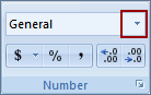
- With the cells to be formatted all selected, click the arrow in the format dropdown box in the Number group on the Home tab. (The default option is
General.) You’ll notice a list of format types appear. Select Currency. Each of the cells included in the selection are now formatted to the currency format, or $80,000.00.
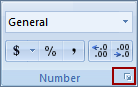
In our example we formatted the numbers as currency. By clicking the small arrow on the lower right corner of the Number group, you will notice the Format Cells dialog box. From here you have greater formatting options, including the number of decimal places and the appearance of negative numbers.
Creating a Chart
Charts are visual representations of worksheet data. Various types of charts can be created in Excel, such as bar, line, and pie charts. Charts can be used to clarify trends or relationships that might not be apparent in the worksheet data alone. Once a chart is created, as data points on the worksheet are updated, the chart automatically changes to reflect those updates.

To demonstrate charting data, let’s consider the illustration above. We have a worksheet that contains data cells on the left and those same data cells charted on the right. To chart the data cell range L9:N14, do the following:
- Using the illustration as your source, type the numbers and headings into a blank worksheet starting at cell L9. You will only type the data included in the range of cells starting at L9 on the top left to N14 on the bottom right or data range L9:N14. The chart to the right is what we’re about to create. Try formatting the data as shown to practice what has already discussed, and remember to input “plain” numbers and format using Excel’s formatting tools. (TIP: 16 = 1600%, .16 = 16%)
- One you have completed the data entry, select the range L9:N14 by clicking cell L9, holding the mouse button and dragging down and to the right until you reach cell N14.
- With the cell range highlighted, click the Insert tab on the Ribbon at the top of the Excel screen, and in the Charts group click Line. You will notice an option box appear presenting various line chart style options. Select the top left 2-D Line style. When you click this option, the line chart is inserted onto the worksheet.

Once you’ve inserted the chart, notice that the tab on the Ribbon at the top of the screen has switched from the Insert tab to the Chart Tools Design tab. Within Chart Tools, you have an assortment of options including chart style, layout, and format. However, for our purposes, the default styling of the inserted chart works well.
Printing the Worksheet
Page Setup

To prepare a worksheet for printing, Excel offers several options to control how it will appear on the printed page. It’s always a good idea to review the layout before printing—checking for things like orientation and margins—to verify that the worksheet will print as intended.
To do this, select the Page Layout tab on the Ribbon at the top of the Excel screen. From there, notice the Page Setup group which includes options to control page orientation, margins, and paper size, among other things. Click on each option and select the parameters you desire.
Note the Print Area button in the Page Setup group. If you have a worksheet that has multiple components to it and you wish to print those components separately, you can define specific areas or cell ranges of the worksheet to be printed, ignoring the other areas.
Print Preview


It is a good idea to always preview before you print so that you can make any adjustments before printing and save yourself repeated attempts and wasted paper. To preview what you’re about to print, click the Microsoft Office Button at the top left of the screen, click the arrow next to Print, and then click Print Preview. From in the Print Preview page, notice the Page Setup button in the Print group on the Ribbon. By selecting this option, you have control over all of the Excel page setup options.
Printing
Once the worksheet has been prepared for printing, it can be printed by selecting the Print button in the Print group on the Ribbon within Print Preview, or by clicking Print from the Microsoft Office button.
Saving the Worksheet

You should save your work frequently. If you have a power outage or some other problem, you can start working again from your last saved version.
When you create a new worksheet and save it for the first time, you are always asked for a name to assign to the worksheet. Click the Microsoft Office Button at the top left of the screen and then click Save. If the worksheet is new, a dialog box will appear asking for a name and location to save the worksheet. If the worksheet you are working on as been previously saved, clicking Save will save a new copy of the previously named worksheet overwriting the previous version.
If you would like to save an existing worksheet to another name, thus keeping the original version in its original condition, click Save As. A dialog box will appear asking for a name and location to save the new worksheet.
What Next?
The purpose of this overview is to give a general understanding of some basic features of Microsoft Excel. By no means is it comprehensive. There are several places to go to learn more about Excel.
You might start by taking advantage of the tutorial features available within Excel itself. From Excel Help, search for “tutorials.” In addition, online help is quite extensive and is best used for finding information quickly. Use your favorite Internet search engine to find answers.
Also, if you would like specialized information, there are many comprehensive books available.
This overview was developed by Dr. Sharon Garrison.
No adaptation of its content is permitted without permission.
FAQs
1. What is Excel?
Excel is a spreadsheet program that allows you to organize, compute, and analyze text and figures. When you use formulas, any changes to the original values are immediately recalculated throughout the whole spreadsheet.
2. How is Excel used in finance?
There are many things that you can do with Excel. In finance, it is often used to track and analyze data. For example, you might use Excel to create a budget or to track your investments. It can also be used for more complex tasks such as financial modeling.
3. What are the top financial Excel functions?
There are many things that you can do with Excel. In finance, it is often used to track and analyze data. However, there are basic things that you can do in any version of Excel: Create and manage worksheets, Enter text and numerical data, Perform mathematical operations, Format cells and data, Print workbooks and individual worksheets, and basic functions in Excel.
4. What are the 7 basic Excel formulas?
There are seven basic functions in Excel: SUM, AVERAGE, MIN, MAX, COUNT, COUNTA, and LARGE. All of these functions are located on the Home tab in the Editing group.
5. What is the most useful tool in Excel?
There is no one-size-fits-all answer to this question. However, some of the most commonly used tools in Excel include the SUM function for adding data, the AVERAGE function for computing averages, and the COUNT function for counting numbers. Many people also find the PivotTable tool to be extremely useful.